
How to: Mosaic Plots
What is a Mosaic Plot anyway?
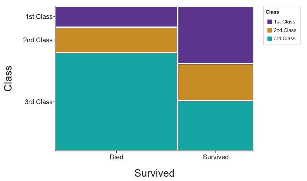
The Mosaic plot shows the distribution of categorical values in a 2D array, which can be a good way to convey insights about the dataset.
Each tile’s area is proportional to the number of cases in that combination. Column widths show how the X variable splits up (3rd class was the biggest group), and tile heights within each column show how the Y variable splits within that group (most 3rd-class passengers died). If the two variables were unrelated, the horizontal lines would line up across every column.
How do I make a Mosaic Plot?
Selecting Variables
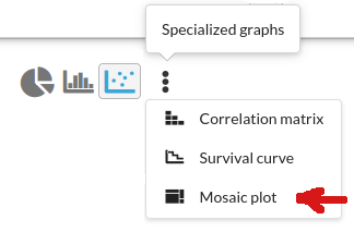
On the graph tab, go to Specialized graphs -> Mosaic plot:
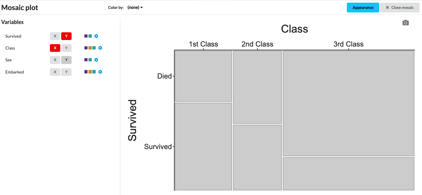
This will switch you into the Mosaic view, where you can select which columns of categorical data you want to apply to your axes. Click X to split the plot into columns by that variable (divides along x-axis), and Y to split each column into tiles (divides along the y-axis). The plot starts gray until you add color.
Adding Color
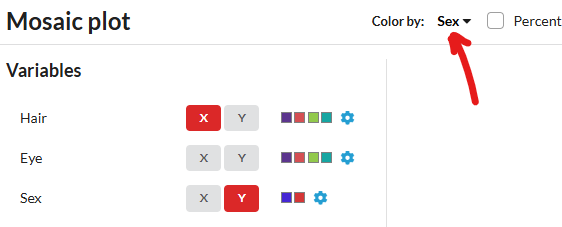
You can choose to color by one of your variables, using the Color by option. The colors it uses are the ones selected for the values of your categorical variables (same as Customizing categorical variables) and you can change them via the small gear icons.
Below you can view two examples with the same variables plotted, but a different variable chosen for color:
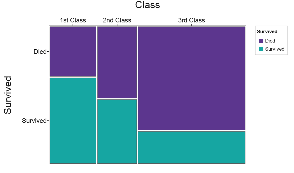
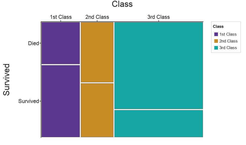
Coloring by Survived makes survival rates easy to compare across classes. Coloring by Class only repeats what the columns already show. Students should color by the variable whose pattern they want to highlight
Color by Residuals
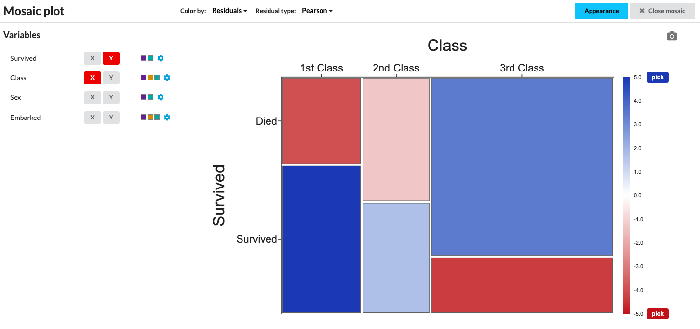
Alternatively, you can color by residuals. What are residuals? A residual compares each tile to what you’d expect if the two variables were unrelated. Blue tiles have more cases than expected; red tiles have fewer. The darker the color, the bigger the gap. As a rule of thumb, values beyond about ±2 are worth paying attention to.
In the Titanic data, 1st-class passengers who survived and 3rd-class passengers who died are both strongly blue, and 3rd-class survivors are strongly red. Survival clearly wasn’t independent of class.
Which residual type should I use?
Pearson (default): (observed − expected) / √expected. The easiest to explain, and it connects directly to the chi-square test.
Freeman–Tukey: behaves better when some tiles have small counts.
Deviance: each tile’s contribution to the likelihood-ratio (G²) test. It’s the standard diagnostic in statistical software.
For most classrooms, Pearson is the right choice.
Going further:
Looking for even more exciting mosaic plots? You can graph two variables on x or on y for even more complexity for data analysis:
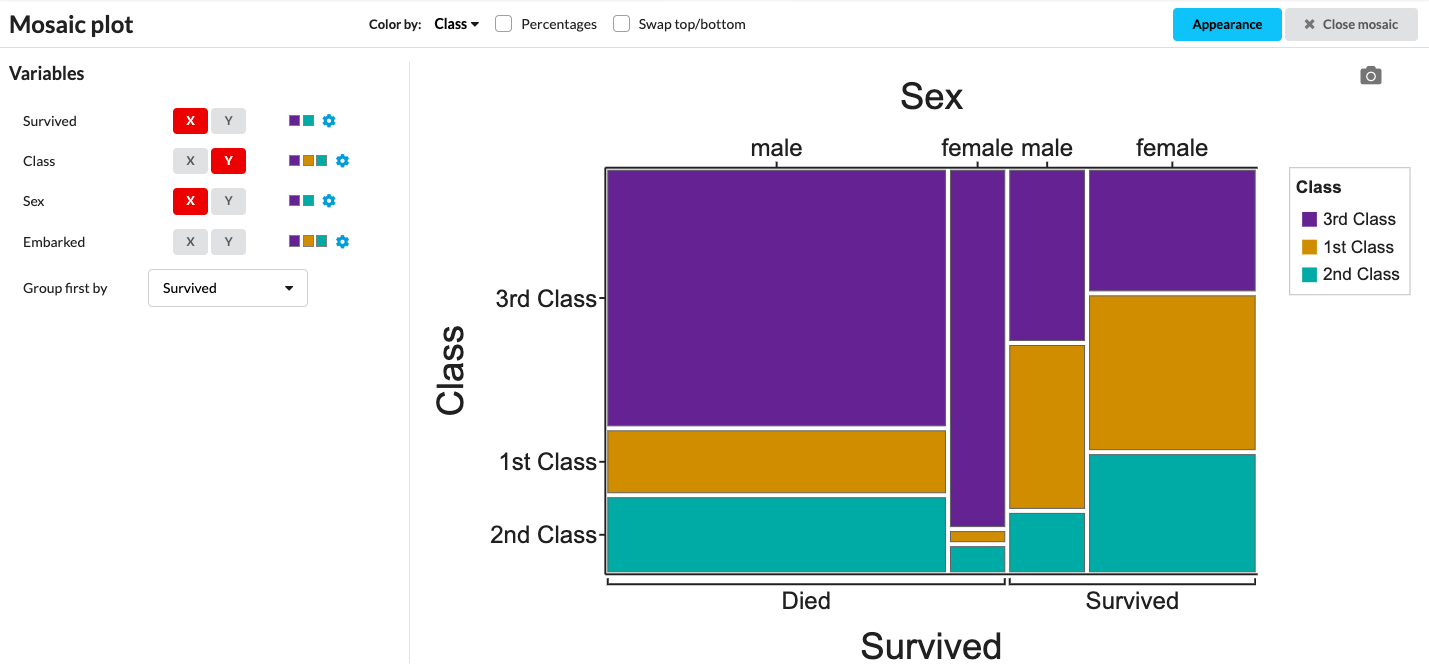
Read more about Mosaic Plots on our User Guide, or give them a try yourself —
here’s our Titanic Manifest Dataset to get you started.