Mitosis in Onion Root Tips
This classic microscope lab has been used in life science classrooms for decades. It is also a standard part of the AP Biology curriculum as Investigation #7 in the AP Biology lab manual, and can be a great way to apply a basic knowledge of chi-square tests.

Background:
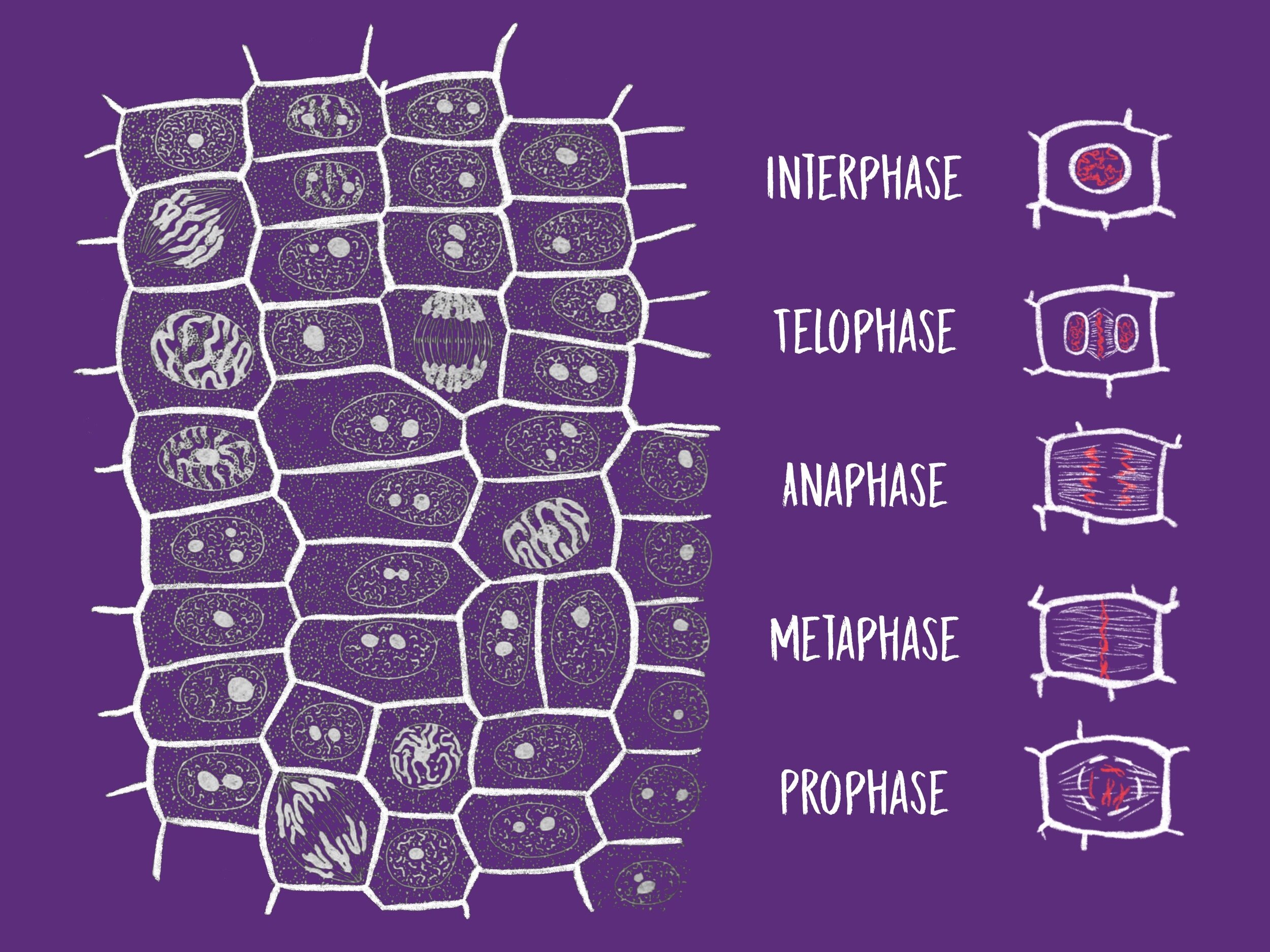
The environment immediately surrounding a cell can have substantial effects on the process of cellular division. Mitosis, one type of cell division, is the process by which a eukaryotic cell separates the chromosomes in its cell nucleus into two identical sets, in two separate nuclei. This is the fundamental process that produces most of the cells in multicellular organisms and allows for growth and repair of an organism.
Fungal pathogens in the soil are known to inhibit root growth in important agricultural plants. These fungal pathogens are thought to act through secreting lectin and lectin-like proteins into the soil to promote mitosis in root tips beyond healthy levels. This artificially high level of mitosis is then thought to damage root tissue, eventually slow overall root growth, and weaken the plant.
In this activity, we’ll use lab data to test the hypothesis that lectin promotes mitosis in onion roots. The two variables for the activity are Phase and Treatment. Each row in the dataset is an individual cell observed with a microscope. Phase corresponds to whether the onion cells were observed to be in “Interphase” or “Mitosis” and Treatment corresponds to whether the onion root tips exposed to lectin (“Lectin”) or not (“Control”).
To test for any statistical effects of lectin on root growth we’re going to use a chi square test of independence. The null hypothesis of this test is that two (or more) variables are independent of one another. In other words, the null hypothesis assumes that there is no predictive ability of one variable on another. In the case of this lab, this would mean that the proportion of control cells in mitosis are similar to the proportion of lectin-treated cells in mitosis. If we find this to be true, then the phase we observe the onion root tip cell to be in would be independent of the lectin treatment and our data would fail to reject the null hypothesis. However, if the proportions of cells in mitosis are significantly different between the control and lectin-treated samples, then we would reject the null hypothesis and conclude that the lectin treatment does affect the proportion of cells observed in mitosis.
In the activity, students will use the “Make-a-graph” feature to find the observed counts of cells in different stages of the cell cycle, and use these observed counts to calculate the expected counts for the null hypothesis. They may then either calculate the result by hand and then use the graph-driven hypothesis test to check their results or simply complete the test by hand (the graph-driven chi-square test for independence is a paid feature, but you can start a 90-day free trial to create classes and give your students access).
Dataset
To collect this dataset, both lectin-infused roots and non-exposed lectin root tips (control) were observed using microscopes. While looking through the microscope at a root tip on a stained slide, cells were observed and for each cell it was noted whether that cell was in interphase or undergoing mitosis. Because the cells were preserved in whatever stage of the cell cycle they were in when the slide was prepared, the slide is like a snapshot of what was happening in that root tip at the time of collection.
The null hypothesis is that results will show no difference between the control and treated groups in terms of the time spent in mitosis relative to interphase. The alternative hypothesis is that the lectin treatment will increase the amount of time that cells in the root tip spend in mitosis relative to the time spent in interphase.
Variables
Phase: This is a categorical variable with two values. Each observed cell was either in Interphase or Mitosis.
Treatment: This is a categorical variable with two values. The root tip and its cells were either treated with Lectin or a Control (not treated).
Activity:
1) Use the “Make a graph” feature to make a categorical bubble plot (accessible with the scatter plot icon) to compare the relative proportions within each group. Show Treatment on X and Phase on Y. Screenshot your graph below, and answer the question: What does the graph seem to suggest about the impact of lectin on onion root cell metabolism?

2) Given that a p-value of .05 or below indicates a strong evidence that lectin does impact cell growth, give your best estimate for the p-value for a Chi-Square Test of Independence. Without actually doing any calculations, do these results look like a significant deviation from the null expectation for the same proportion of cells in mitosis in both treatment groups?
3) With DataClassroom: Use a graph-driven chi-square test for independence* to have the computer do the calculation. After you have made the graph, just click the Graph Driven Test Button (on the right panel just left of the Appearance button). How close was your estimate of the p-value to the actual calculated value?
By Hand: Determine if there is a statistically significant difference between the observed frequency of cells in interphase and mitosis between the two treatment groups. To do so you will need to do the following:
a) Calculate the expected values assuming independence. For an in-depth explanation of why we calculate independence this way, please see the Teacher’s Note below. (Hint: e1 should be around 71.75)
N = total number of cells in the experiment
e1 = expected value of cells in the control group in interphase = all cells in interphase * all cells in the control group / N.
e2 = expected value of cells in the control group in mitosis = all cells in mitosis * all cells in the control group / N.
e3 = expected value of cells in the treatment group in interphase = all cells in interphase * all cells in the treatment group / N.
e4 = expected value of cells in the treatment group in mitosis = all cells in mitosis * all cells in the treatment group / N.
The table below is a helpful way to organize this information (a modified version of the one provided under Investigation 7 in the AP Biology Lab Manual):

b) Calculate chi-squared statistic using the following formula:
Χ2=Σ(o-e)2/e
“o” is the observed count for each category you found in 1), and “e” is the expected count you calculated in a). Make sure each “e” and “o” correspond to the same category. The table below is a helpful way to organize the information. (Hint: the first of the four values you’ll find and add should be 2.089)

c) Compare the chi-squared value to a table of critical values for the chi-squared distribution.
*DataClassroom only has a Chi-Square Test of Independence so we use that here in place of the more appropriate Chi-Square Test of Homogeneity. The difference between these two tests is not in the calculation, but rather in the experimental design and sampling method. Quantitatively and qualitatively the conclusions drawn will be the same.
Teacher’s Note
Chi-square tests can be daunting, especially for high school students without a background in statistics, but they’re really useful for analyzing datasets with categorical variables. Although these are frequently taught by hand, students should understand that these tests are almost never performed by hand in the real world. Scientists rely on computers to perform statistical tests, but ideally have a thorough understanding of how tests work and how their results can be interpreted.
All Chi-square tests are looking to see if there is a big enough deviation from expected counts, based on the assumptions of the null-hypothesis, to conclude that those assumptions that gave us the expected counts are not true. If the observed data differ enough from the expected values we reject the null hypothesis.
A quick breakdown of different types of chi-square tests:
Goodness of fit: used when there is a known, discrete distribution. Rolls of a dice or coin flips are a great example of instances when goodness of fit would be appropriate.
Test for independence (used in this activity): used to determine whether two different categorical variables are associated with one another.
Test of homogeneity: when data is collected by randomly sampling each subgroup of a categorical variable separately.
Let’s focus on the tests for independence, since the calculations when we assume independence can be a little tricky. For a these tests, our expected counts are calculated by multiplying the ratio of all observations in the dependent variable category (cell phase, in this case, divided by N, the total number of observations) by the number of elements in the independent variable (treatment) category. If this value is close to the observed number of a dependent variable in an independent variable category, then the impact of the independent variable on the dependent variable would be negligible, and the two variables are thought to be independent.
Chi-square tests have interesting distributions that change with the number of variables studied. Here is a chart of critical values for chi-square distributions with different degrees of freedom. The numbers in the table are chi-squared values for which the probability of the the null hypothesis being true based on the outcomes of a test are the values at the top of each column. For instance, if you conducted a test with 2 degrees of freedom (“df”) and calculated a chi-squared value of 5.991, there’d be a only a 5% chance of obtaining data that differed from the null expectation by that much through random chance . As you can see, when more variables are considered, there needs to be greater deviation from our expected values in order to reject the null hypothesis.
