The Stroop Effect Part 2
Can you ignore incongruent information?
Analyze a classic experiment in psychology with this dataset based on the original 1935 paper by John Ridley Stroop. Activities from Stroop’s original datasets are spread across 3 separate activities, it is recommended that you complete them in sequential order to get the most out of them.
Part 1 - How does color interference affect reading time?
Part 2 - How does word interference affect reading time?
Part 3 - How does practice influence interference?
Background

For more information on Stroop Effect, check out part 1 before proceeding.
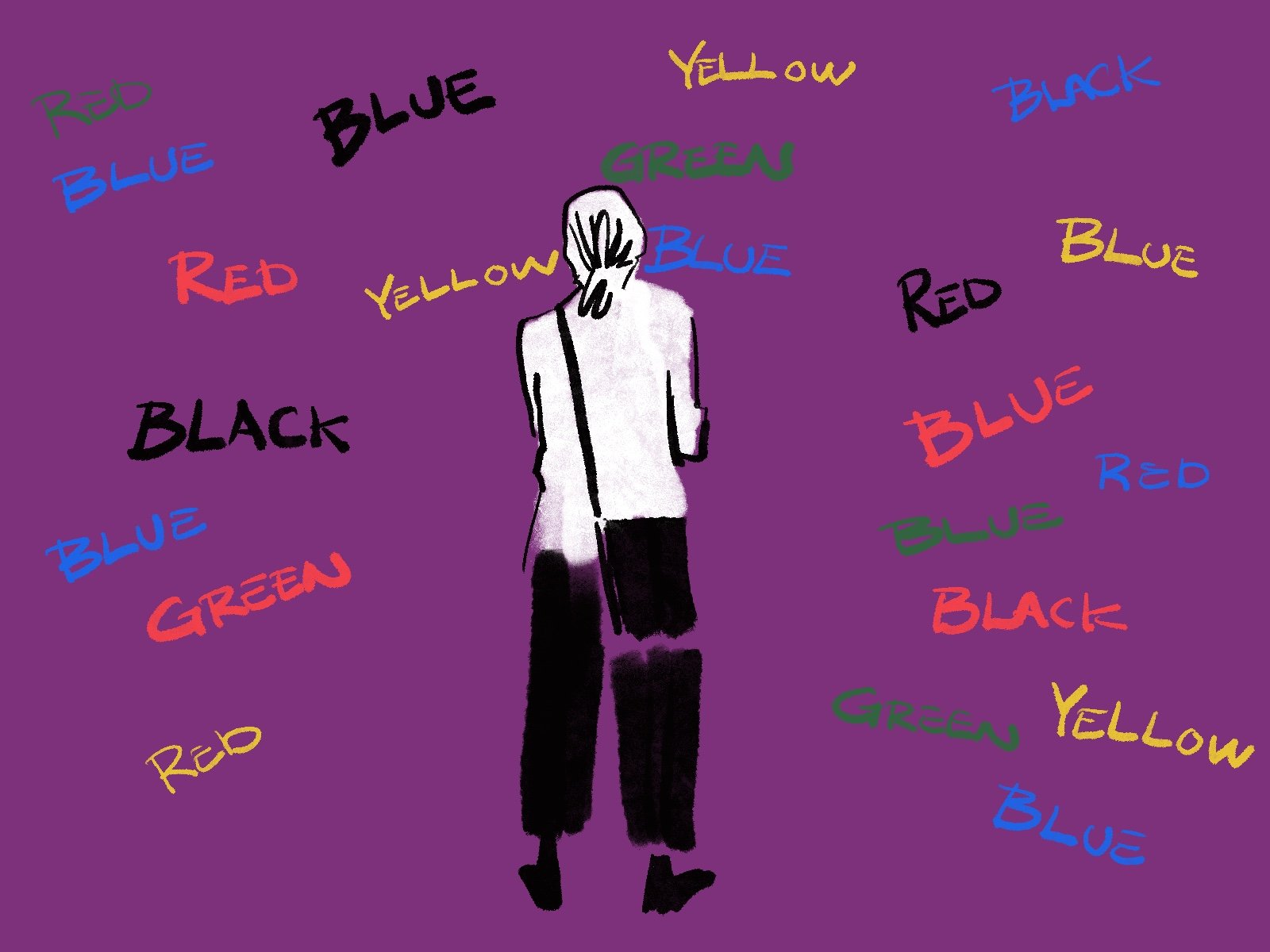
If you thought reading the color names was difficult in the list (right), try naming the physical color for which words are written on the left and then on the right.
Did you find yourself taking even longer when naming the colors in which words are written on the right side and sometimes saying the wrong color altogether? Could the interference due to conflicting words be even stronger when trying to name the colors in which words are written as opposed to reading the words itself when they are written in conflicting colors (part 1)? Stroop thought that this would be the case given that we typically learn and process words and their meanings earlier than we process their visual connotation which in the case of colors tends to be more abstract.
Analyze the data below on your own and compare it to what Stroop found in his study in the second experiment he performed.
Dataset

In his second experiment, Stroop had participation from 100 college students (29 men, 71 women). Each was given a sheet in which each square was shaded in a different color. He recorded the time it took for participants to identify the colors of each square in order. Then, using the same list he provided students in Experiment 1 (RCNd), he now asked students to name the color in which words were printed. Here, the words were always printed in a color different from what the word indicated.
When students made errors in each list they were allowed to correct it. If not corrected, extra time was added to their total time taken to read the list (the amount added was equal to twice the average time per word of the sheet on which the error was made). An increase in time would indicate the presence of word interference. Stroop also predicted this interference (due to words in naming colors) would be greater than the interference from Experiment 1.
Variables
Participant ID: This info variable is a unique ID given to each participant. This variable will not be analyzed
Sex: This categorical variable indicates whether the participant was male (M) or a female (F)
Year of Study: This categorical variable indicates whether the participant was in undergraduate (1st-4th Year) or Graduate school
Time to Read (s): This numeric variable is the time it took for a participant to read the associated word list measured in seconds. It includes any added time for missed words.
Treatment: This categorical variable is the type of word list that participants will have to read in a given experiment: Naming colors of squares (NC) or Naming colors of the words written in ink different from the one they refer to (NCWd).
Time to Read - Simulation 2 (s): This numeric variable is thetime it took for a participant to read the associated word list measured in seconds. This variable is to be used for the simulation section only.
Activity
1) State the question that Stroop asked, below:
2) What was Stroop’s hypothesis of this experiment?
3) What variables would you need to explore the question? State your prediction of those variables below:
4) Make a histogram of time to read as x-variable (number should appear as your y-variable). Set treatment as you z-variable. Screenshot your graph below:

5) Add a normal distribution, as well as median-based descriptive stats to this group. Screenshot your graph below:

6) To fully understand the data, we need one more graph for comparison. Display the dotplot of Time to Read as your y-variable and treatment as x-variable. IncludeAdd descriptive statistics for their mean and 95% confidence intervals. Include your screenshot below:

7) Does the interference of different words seem to affect the ability of participants to name the colors those words? Reference data from the previous graphs (#5 or #6) to explain your inference.
8) Run a statistical test to provide further evidence for your answer. Which test is most appropriate?
Record the results below, and explain their significance in context of the Stroop effect.
9) Do males and females differ in their performance in naming colors in the control and treatment? For your scatter plot, Keep treatment as the x-variable, and time to read as the y-variable. Select sex as the Z-variable to indicate reported gender of participants. Select mean and SD to show males and females in each treatment. Screenshot your graph below.

10). Is this difference significant? Run a statistical test on this new graph. Which test was best?
Record the test results below, and explain their significance as evidence for your answer.
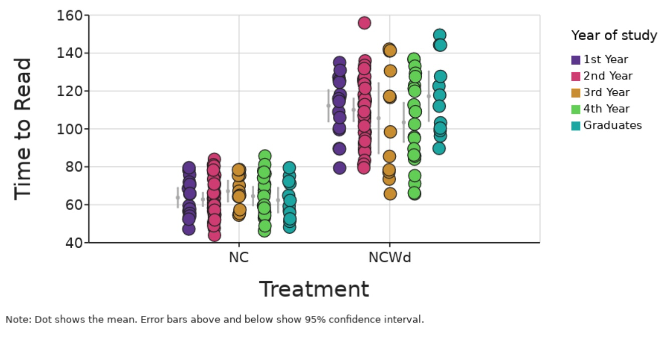
11) Stroop wondered, given the difficulty of identifying colors from words, if the education level of participants influenced their ability to identify color names despite word interference. Do you think reading time decreases or increases with the increasing number of years participants spend in universities? Paste the graph with mean and 95% CIs to test this hypothesis. Explain if the data supports your claim or not? (Hint: 95% CIs which overlap mean values of other groups typically indicate non-significant differences between groups)
12) Based on your work in parts 1 and 2 related to the Stroop dataset, answer the following:
Which form of interference is stronger - that due to color or words? Point to specific pieces of evidence to explain your claim.

13) Explain what the relevance of conducting a post-hoc test might be for an analysis comparing the effect of both treatment and sex on reading time.
Report post-hoc test results below and explain how your interpretation changes regarding the effect of sex on reading time.
Part 1: Use our simulation data
14) The post-hoc test indicated that the difference among males and females in reading ability was stronger between treatments rather than within a treatment. Stroop had only 29 male participants as opposed to 71 female participants in his study, and the standard deviations around the mean were fairly large. Using the simulation tool we generated a new set of reading times for males and females in each treatment (using the same mean and SD) of this experiment in a column titled “Time to read - Simulation 2”). Set this variable as your new y-variable (with treatment as x-variable and sex as z-variable). Screenshot your graph below:

15) What do you see with this new data? What does it tell you about the replicability of the treatment effect as opposed to the effect of Sex? (Run another statistics test to provide further evidence).
Part 2: Make your own simulation data
16) Create a new dataset for only Experiment 2, and try analyzing the data again with respect to sex and treatment, using data from a simulation model you create using the mean and SD either calculated from this dataset or derived from Stroop’s original study. However, now sample 25 males and 25 females for each treatment, thus getting a balanced experimental design. (Hint: Using the sample simulation model, create your own copy and modify the % samples from each sex to be equal)
Create a graph with time to read as the y-variable, treatment as x-variable, and sex as a Z-variable. Screenshot it below:
17) Do you get the same results as Stroop’s paper with respect to sex differences in the time it takes to identify colors? Use information from tests of significance to support your discussion.

*Teachers can request an answer key through the form below.